Project URL in R: Customer_Lifetime_Value_Analysis.notbeook-in-R.html

Tools used: RStudio, Microsoft Excel, Power Query, Tableau

Section 1: Introduction to the project

Problem description

Customer retention is a key challenge for businesses, and understanding the lifetime value of customers (Customer Lifetime Value, CLV) is crucial for developing effective retention and growth strategies.

IBM Watson Analytics company wants to make informed decisions about customer acquisition, retention, and development to optimize resources and maximize profitability.

Business Objective

"Create a predictive model that considers the provided demographic and purchasing behavior data to estimate the Customer Lifetime Value, and improve customer retention programs."

Sección 2: Data Description

Features to be provided for model development

For the project, historical data was provided in a .csv file with 24 columns and 9134 observations. This file contains various demographic characteristics, behavior, policy information, and vehicle details of the customers.

Columna	Type of data	Subtype of data	Ranges o Categories
1. Customer	Categorical	Nominal	ID de 7 caracteres que combina números y letras
2. State	Categorical	Nominal	Arizona, California, Nevada, Oregon, Washington
3. Customer Lifetime Value	Numerical	Continuous	1,898.00 a 83,325.38
4. Response	Categorical	Nominal	Yes, No
5. Coverage	Categorical	Ordinal	Basic, Extended, Premium
6. Education	Categorical	Ordinal	Bachelor, College, Doctor, High School or Below, Master
7. Effective to date	Numerical	Discrete	1/1/2011 a 2/28/2011
8. Employment Status	Categorical	Nominal	Disabled, Employed, Medical Leave, Retired, Unemployed
9. Gender	Categorical	Nominal	F, M
10. Income	Numerical	Continuous	0 a 99981
11. Location code	Categorical	Nominal	Rural, Suburban, Urban
12. Marital Status	Categorical	Nominal	Divorced, Married, Single
13. Monthly Premium Auto	Numerical	Continuous	61 a 298
14. Months Since Last Claim	Numerical	Discrete	0 a 35
15. Months Since Policy Inception	Numerical	Discrete	0 a 99
16. Number of Open Complaints	Numerical	Discrete	0 a 5
17. Number of Policies	Numerical	Discrete	1 a 9
18. Policy type	Categorical	Nominal	Corporate Auto, Personal Auto, Special Auto
19. Policy	Categorical	Nominal	Corporate L1, Corporate L2, Corporate L3, Personal L1, Personal L2, Personal L3, Special L1, Special L2, Special L3
20. Renew Offer Type	Categorical	Nominal	Offer1, Offer2, Offer3, Offer4
21. Sales channel	Categorical	Nominal	Agent, Branch, Call Center, Web
22. Total Claim Amount	Numerical	Continuous	0.099007 a 2893.239678
23. Vehicle Class	Categorical	Nominal	Four-Door Car, Luxury Car, Luxury SUV, Sports Car, SUV, Two-Door Car
24. Vehicle Size	Categorical	Ordinal	Large, Medsize, Small

Sección 3: Findings - Exploratory Data Analysis

Coverage vs CLV

Observations

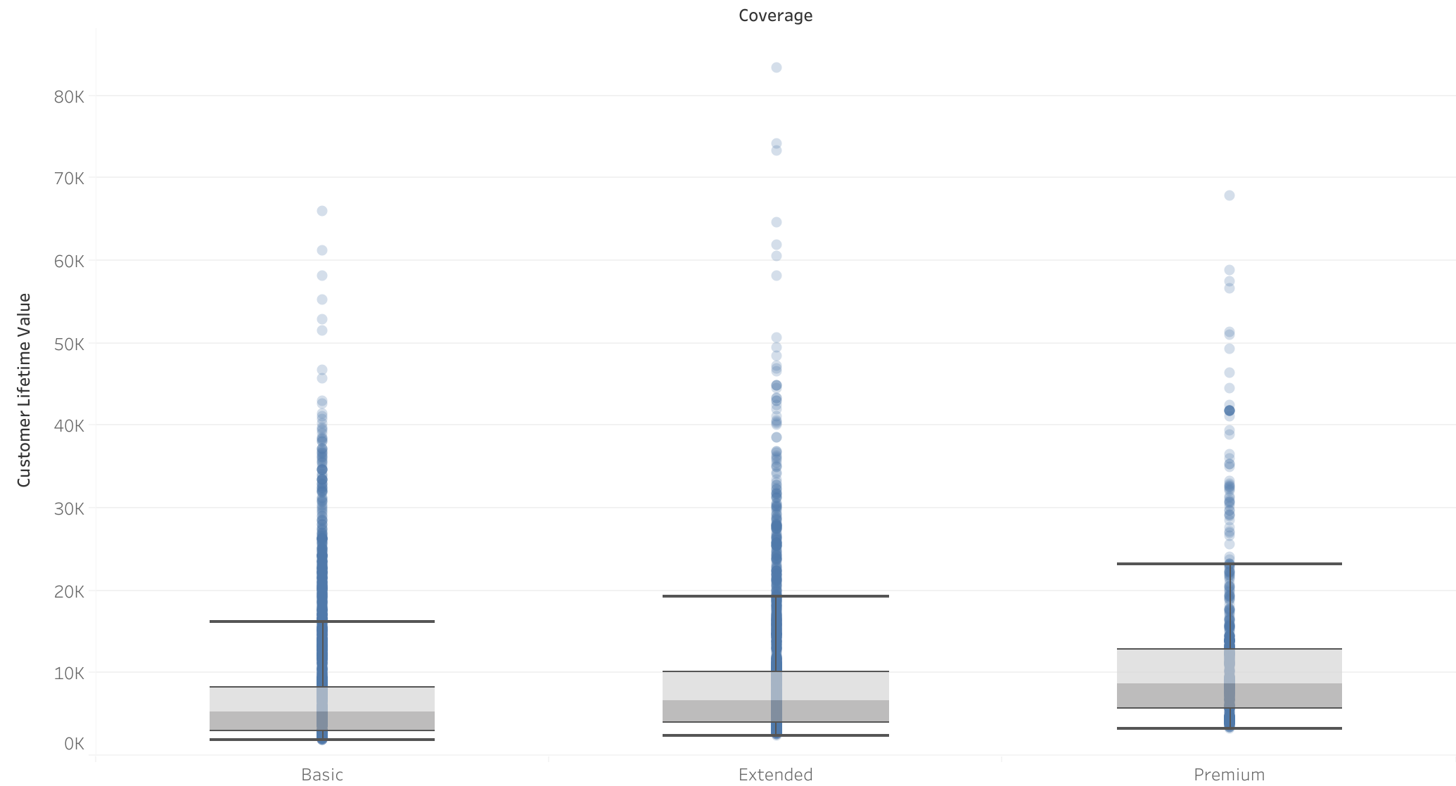
• Correlation between coverage and CLV There is a positive correlation between premium coverage and CLV, as evidenced by the boxplots.

Vehicle class vs CLV

Observations

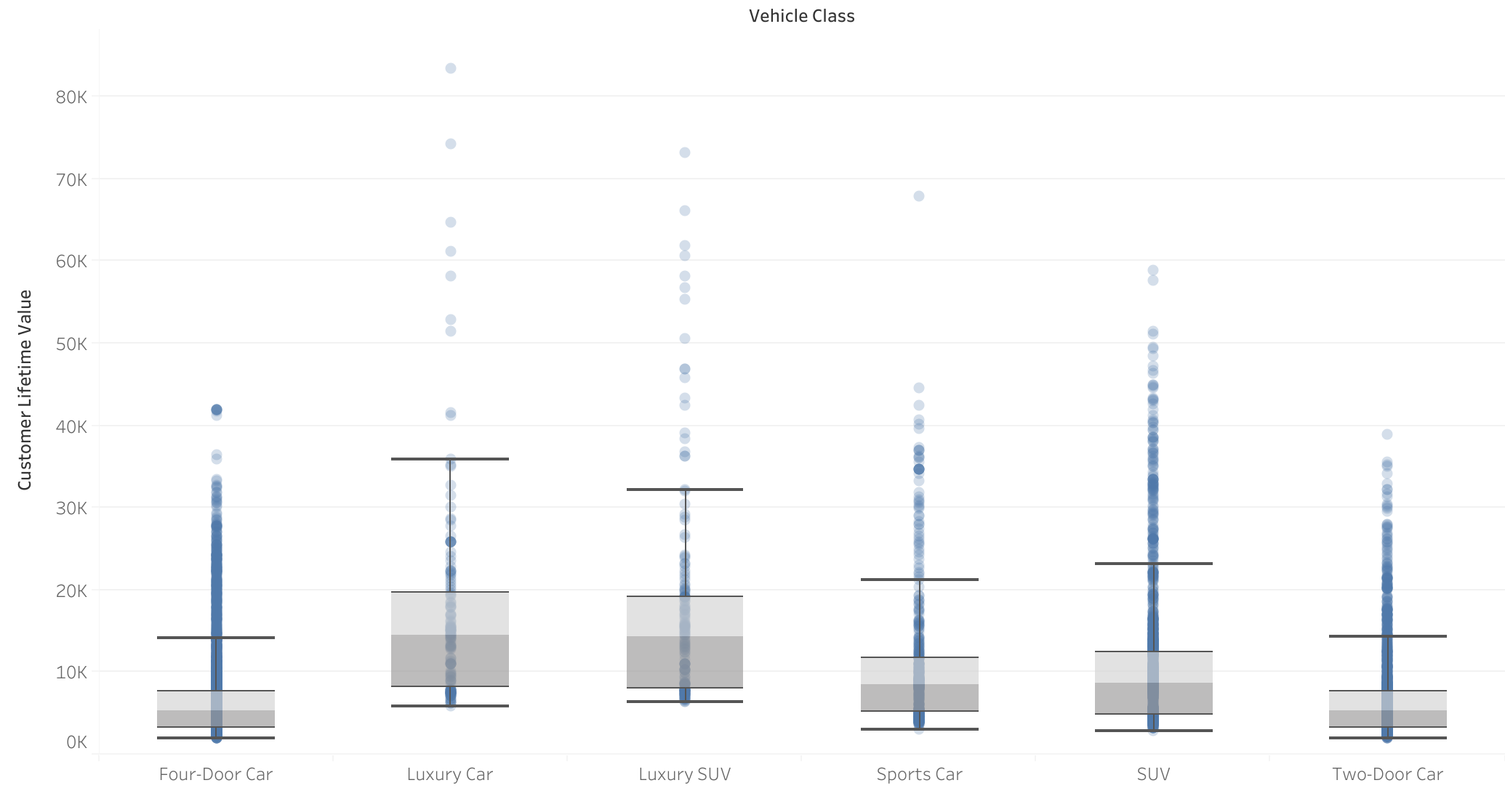
• Correlation between vehicle class and CLV Customers with luxury vehicles have a higher CLV, indicating that the vehicle class has an impact on CLV.

Monthly insurance payment vs CLV:

Observations

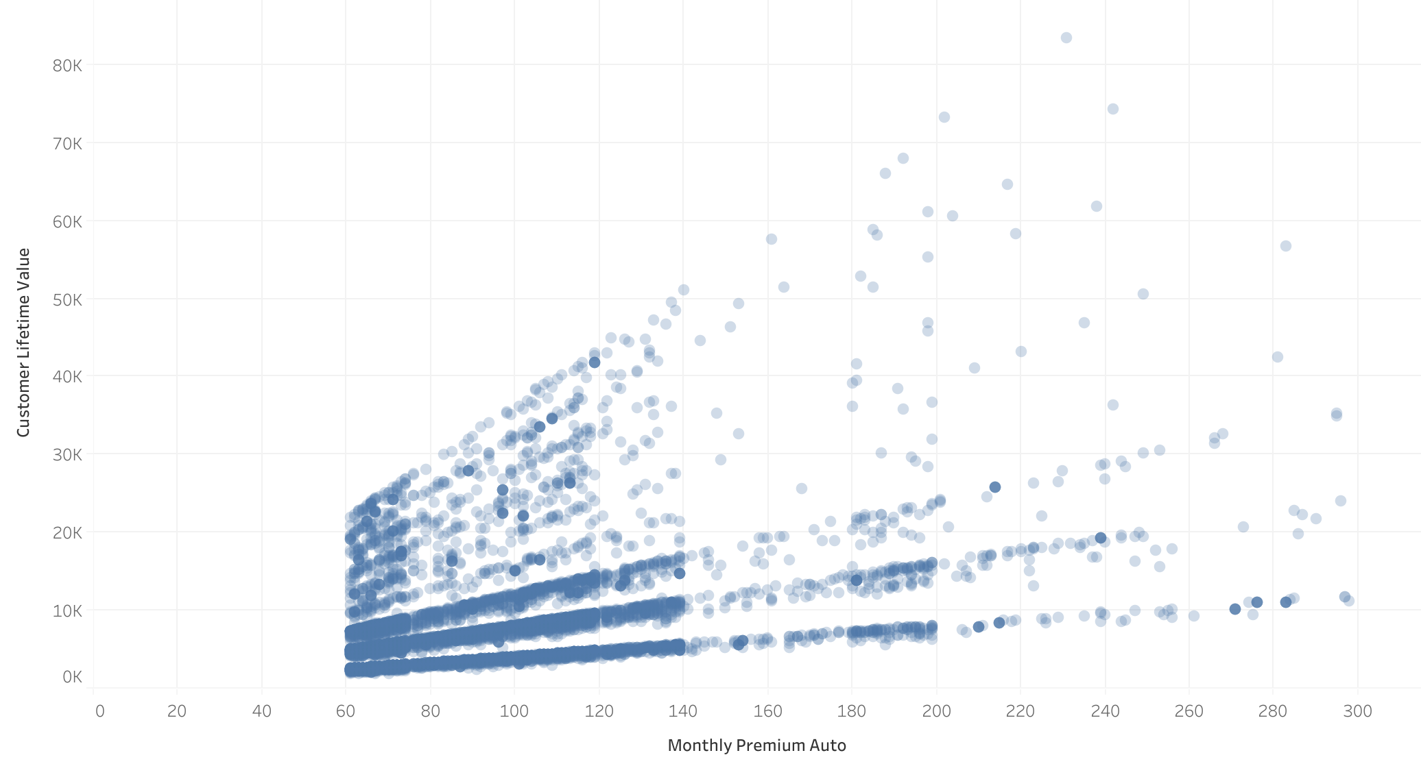
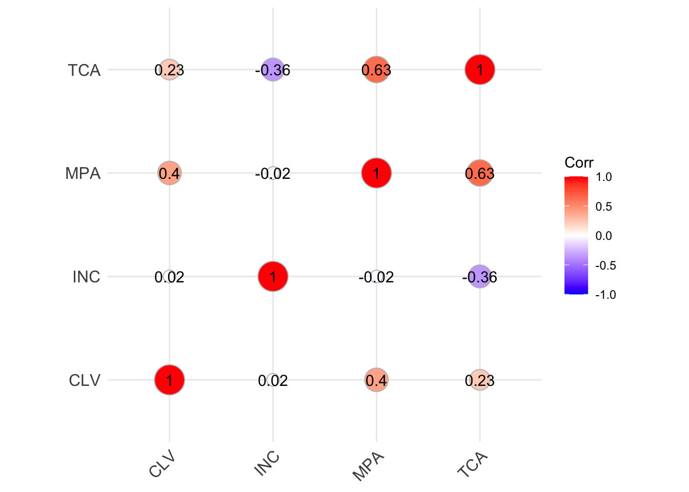
• Highest correlation with CLV: The correlation matrix shows that the monthly insurance payment has the highest numerical correlation with CLV.
• Clear trend in the scatterplot: it is observed that the higher a client's monthly payment, the higher their CLV.

Total claimed vs CLV

Observations

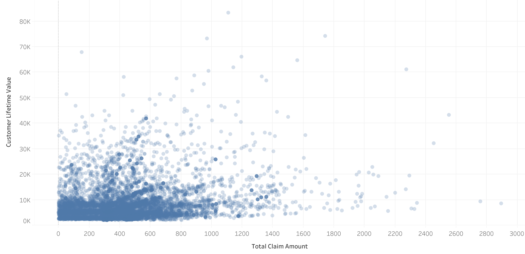
• Correlation between Total claimed and CLV: Although not as evident in the scatterplot, there is a correlation between the total claimed and CLV, corroborated by the simple linear regression model.

Number of insurances vs CLV

Observations

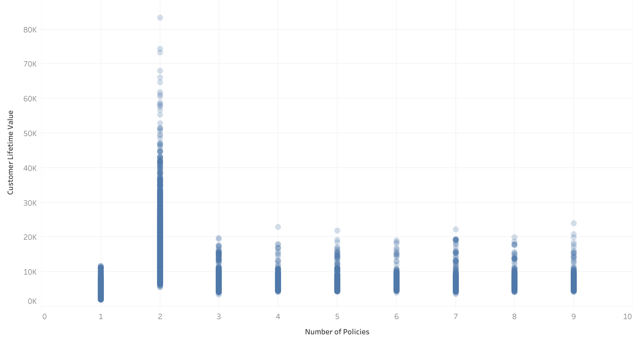
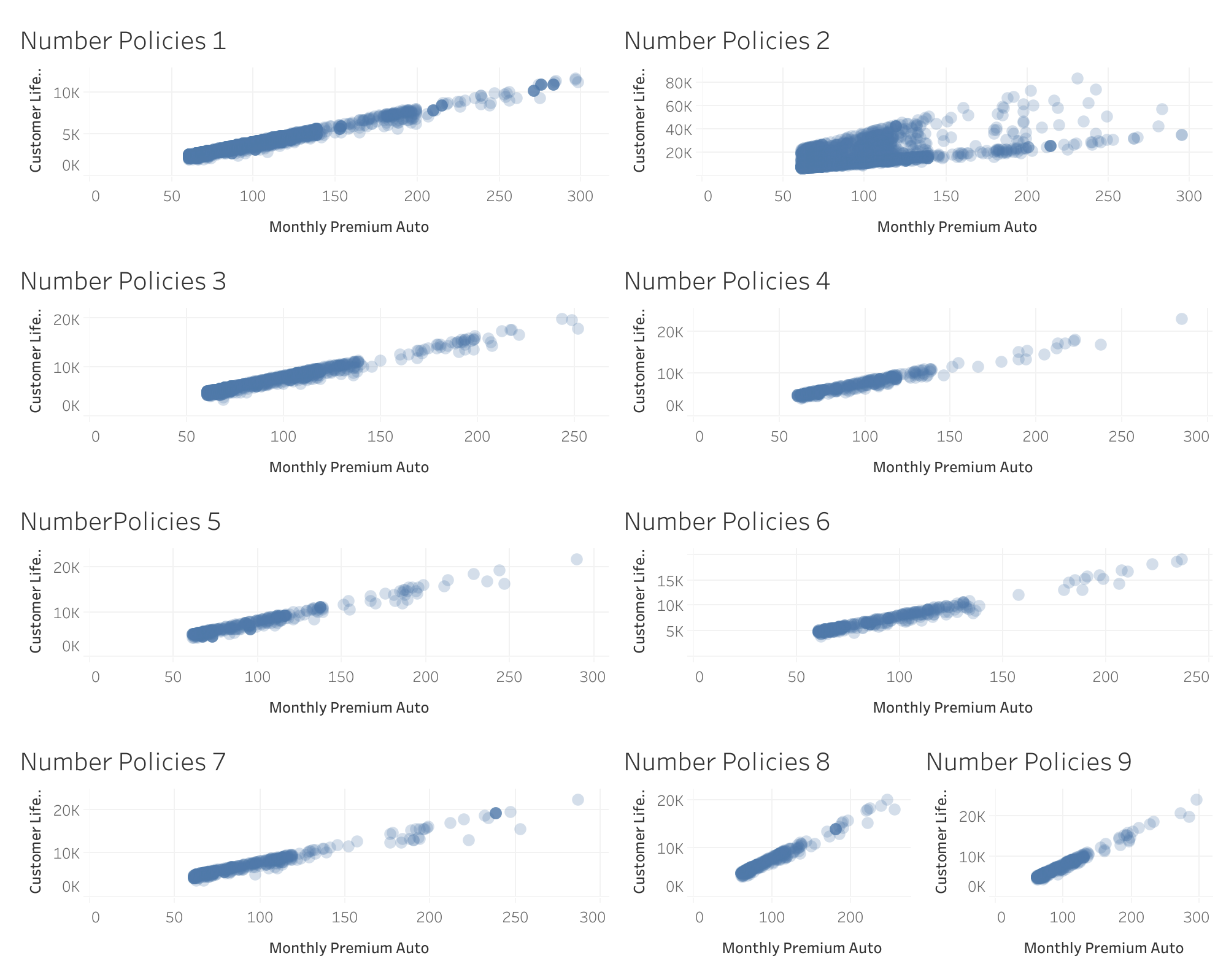
• Atypical increase in CLV for customers with 2 insurances: An unusual increase in CLV is observed for these customers.
• Loss of linearity for customers with 2 insurances: The behavior of clients without 2 insurances is linear.

Section 4: Building the model with Linear regression

Multiple linear regression

Multicollinearity

Multicollinearity was detected in some terms (VIF > 5.0).

Stepwise regression

This method was used to select variables with a greater effect and eliminate multicollinearity.

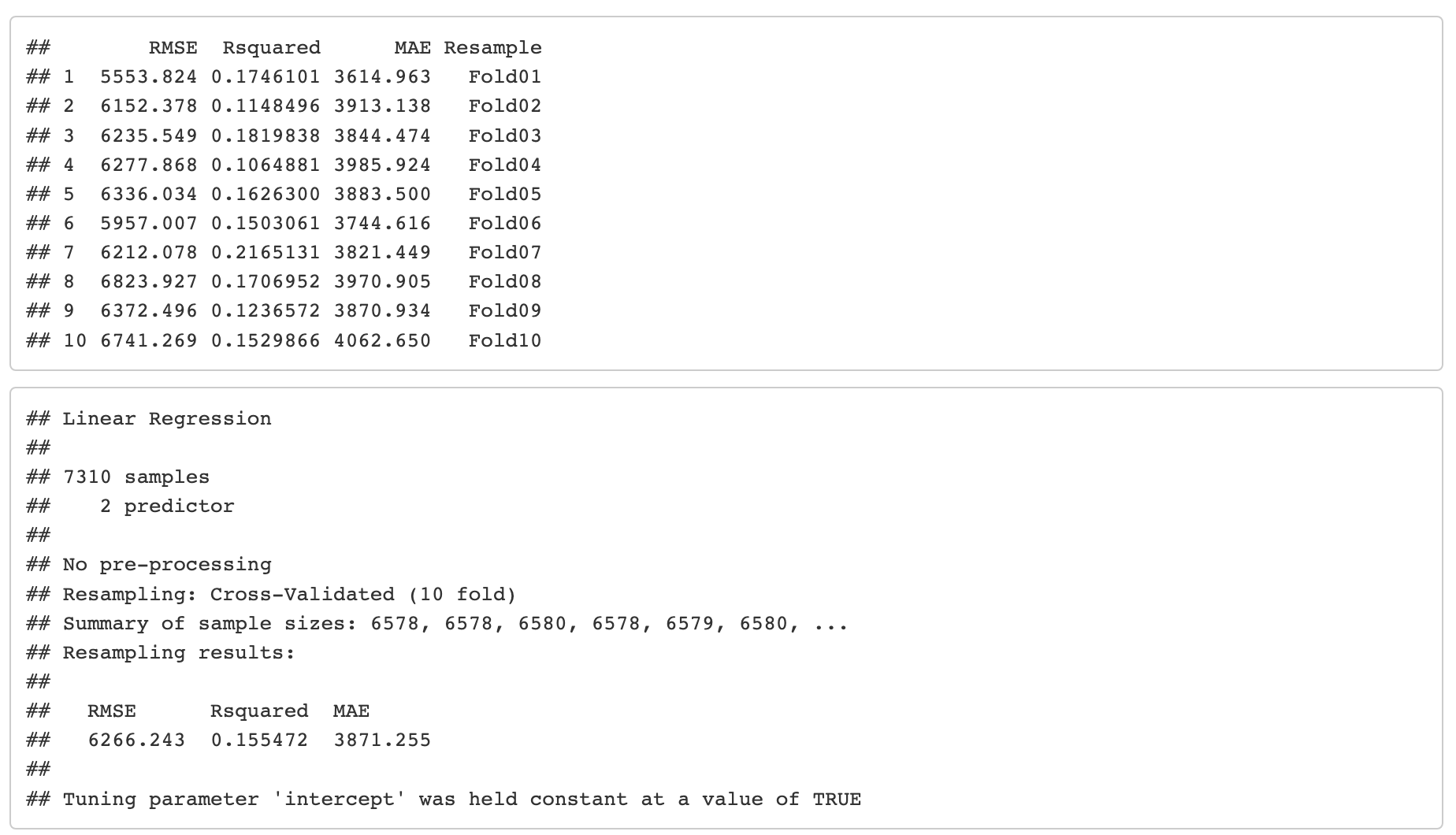
10-fold cross-validation results

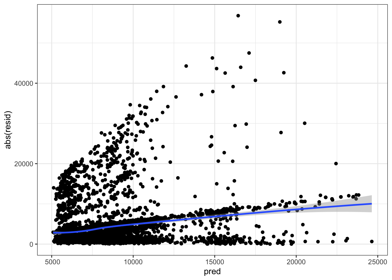
Residuals absolute value VS predicted value

Out-of-sample performance

Section 5: Improving the model with KNN

K Nearest Neighbor.

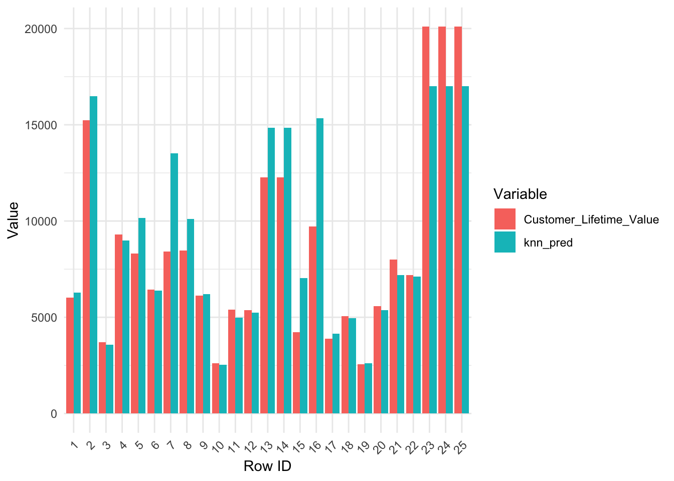
Previously, We found that only when number of policies is 2 the relationship between Customer_Lifetime_Value (target value) and Monthly_Premium_Auto (a feature) vary hugely. We suspect that the model could improve it’s accuaracy by trying using an algorithm that could catch this non linear relationship.

Out-of-sample performance

We get a hugely superior model in the holdout sample.

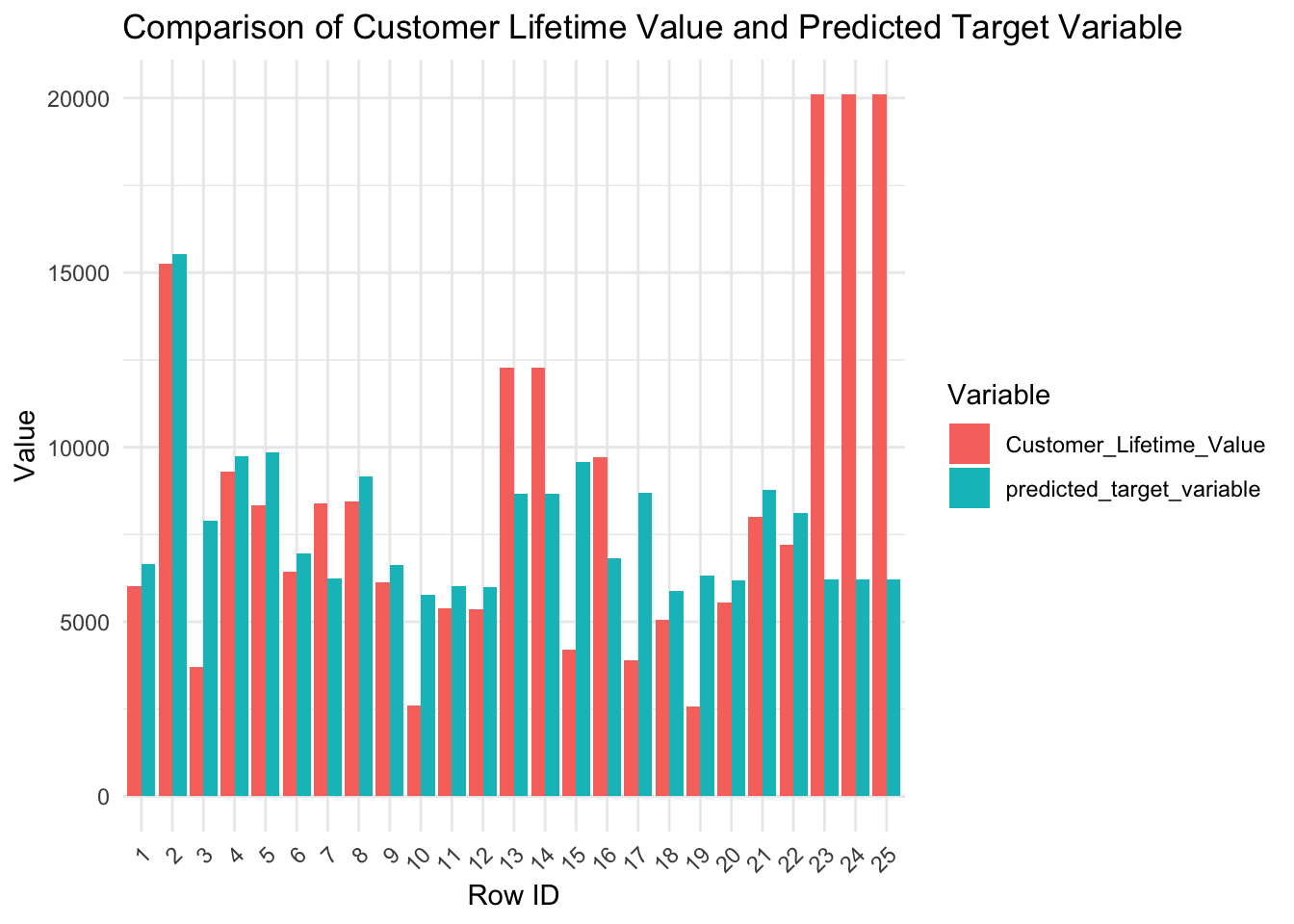
Visualizing Observed vs predicted values on holdout sample

Setting KNN as feature engine

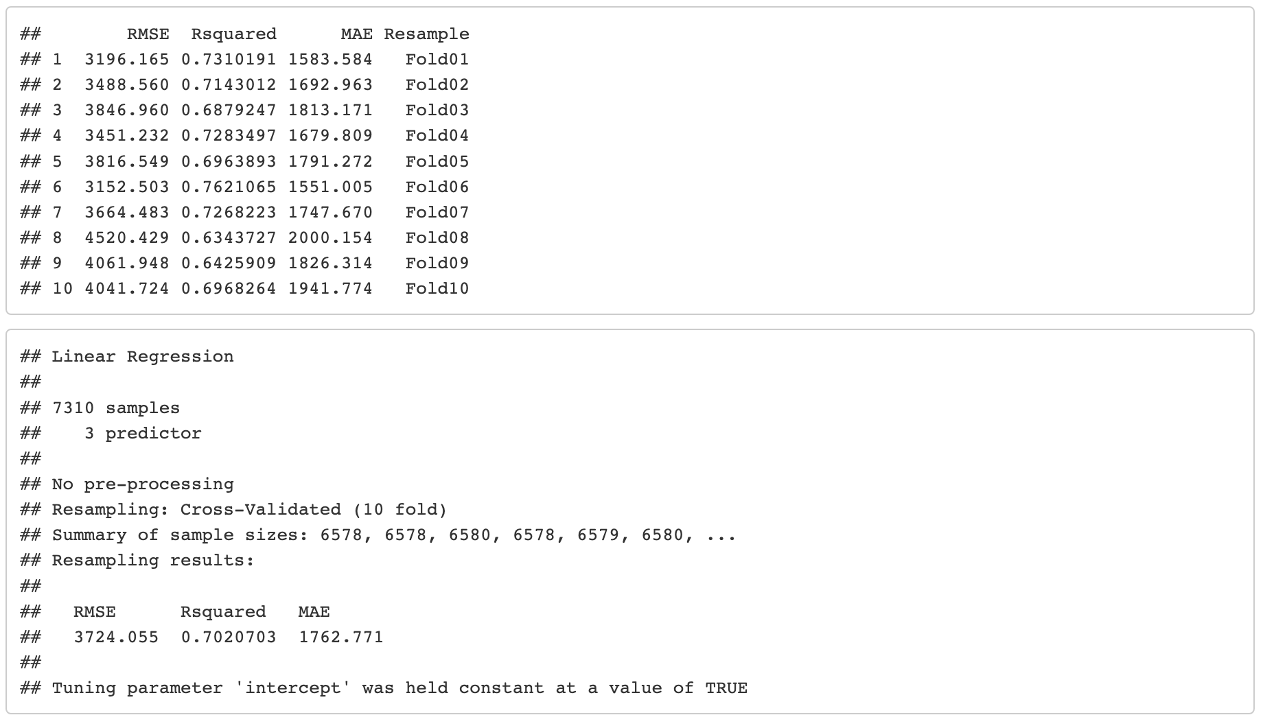
Now let’s try setting KNN as a feature and use it in the multiple linear regression model to see if that could improve the model even further.

10 fold cross validation model

This is a huge improvement. Now we are talking! But let’s not get ahead of ourselves, is important to check other important factors to validate the model like the VIF and most importantly, assessing the model in the holdout sample.

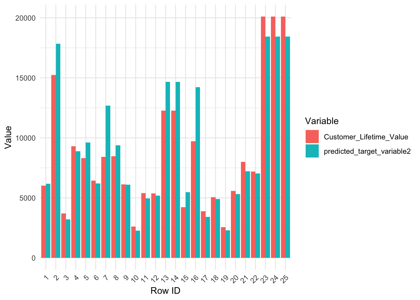
Assessing the model on new data (holdout sample)

Now this is a very good model with a whooping 0.68131 R-squared in the holdout sample.

Visualizing Observed vs predicted values on holdout sample

As it can be seen, the model is very accurate in predicting the customer lifetime value.

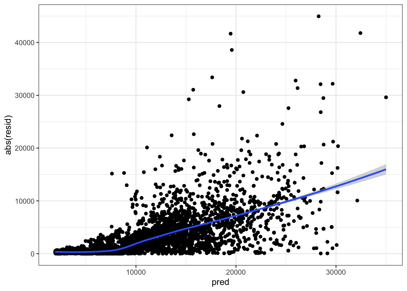
Visualizing the absolute value of the residuals vs the predicted values

Section 6: Conclusion

Our initial linear regression model yielded an out-of-sample RMSE of 6433.889 and an R^2 of 0.1738. Although the model's precision was limited, the insights derived from the coefficients can still be used to inform business decisions aimed at increasing CLV.

The second model significantly improved upon the first by employing an ensemble approach, which incorporated the K Nearest Neighbors (KNN) result as an additional feature. The final model achieved an RMSE of 3994.279 and an R^2 of 0.6813.

The substantial improvement in our model's performance can be attributed to the detection of an unusual pattern among clients holding two policies, which our original linear regression model failed to capture. It is recommended to further investigate this behavior to identify the underlying cause, which may lead to the development of a more accurate model for predicting CLV.